Option Pricing Review
Option pricing
Terminology
T: maturity date
t: current time
\(\tau = T-t\): time to maturity
S: stock price at time t
r: continuous risk-free interest rate
y: continuous dividend yield
\(\sigma\): annualized asset volatility
\(c\): price of a European call
p: price of a European put
C: price of an American call
P: price of an American put
D: present value of future dividends at t
K: strike price
PV: present value at t
ITM: in-the-money
OTM: out-the-money
ATM: at-the-money (K=S)
Price direction of options
- How do vanilla European/American option prices change when those term changes?
| Variable⬆ | European call | European put | American call | American put |
|---|---|---|---|---|
| Stock price - S | ⬆ | ⬆ | ||
| Strike price - K | ⬆ | ⬆ | ||
| Time maturity - T | ❓ | ❓ | ⬆ | ⬆ |
| Volatility - σ | ⬆ | ⬆ | ⬆ | ⬆ |
| Risk-free rate - r | ⬆ | ⬆ | ||
| Dividend - d | ⬆ | ⬆ |
Note: The impact of time to maturity on the European call/put is uncertain.
- If there is a large dividend payoff between two different maturity dates, a European call with shorter maturity that expires before the ex-dividend date may be worth more than a call with longer maturity.
- For deep in-the-money European puts, the one with shorter maturity is worth more since it can be exercised earlier (time value of money).
Put-call Parity
\[ c+K^{-r \tau}=p+S-D \]
American v.s. European options
When the stock pays no dividend, never optimal to exercise American call. Actually, if \[ D_{t} \leqslant K\left(1-e^{-r(T-t)}\right) \] , then it is not optimal to exercise American call. It is possibly optimal for the time right before an ex-dividend date.
Payoff of options
- the payoff of a put is convex function in stock price
- the price of a put is convex function in strike price
Black-Scholes-Merton model
\[ \frac{\partial V}{\partial t}+r s \frac{\partial V}{\partial s}+\frac{1}{2} \sigma^{2} s^{2} \frac{\partial^{2} V}{\partial s^{2}}=V \]
- 推导过程
Feynman-Kac theorem
Let X be an Ito process, given \[ d X(t)=\beta(t, X) d t + \gamma(t, X) d W(t) \] Define \[ V(t, x)=E\left[e^{-r(T-t)} f\left(X_{T}\right) \mid X_{t}=x\right] \] , then \(V(t,x)\) is a martingale process that satisfies PDE: \[ \frac{\partial V}{\partial t}+\beta(t, x) \frac{\partial V}{\partial x}+\frac{1}{2} \gamma^{2}(t, x) \frac{\partial^{2} V}{\partial x^{2}}=r V(t, x) \] and boundary condition \(V(t,x) = f(x)\) for all x.
Under risk-neutral measure, \(dS = rSdt+\sigma SdW(t)\). Let \(S=X\), \(\beta(t,X) = rS\) and \(\gamma(t,X) = \sigma S\) , then the Black-Scholes-Merton differential equation would be \[ \frac{\partial V}{\partial t}+r S \frac{\partial V}{\partial S}+\frac{1}{2} \sigma^{2} S^{2} \frac{\partial^{2} v}{\partial s^{2}}=rV \]
Black-Scholes Formula
Define continuous dividend yield \(y\): \[ c=S e^{-y \tau} N\left(d_{1}\right)-K e^{-r \tau} N\left(d_{2}\right) \]
\[ p=K e^{-r \tau} N\left(-d_{2}\right)-S e^{-y \tau} N\left(-d_{1}\right) \]
where \[ d_{1}=\frac{\ln \left(S e^{-y \tau} / K\right)+\left(r+\sigma^{2} / 2\right) \tau}{\sigma \sqrt{\tau}}=\frac{\ln (S / K)+\left(r-y+\sigma^{2} / 2\right) \tau}{\sigma \sqrt{\tau}} \]
\[ d_{2}=\frac{\ln (S / K)+\left(r-y-\sigma^{2} / 2\right) \tau}{\sigma \sqrt{\tau}}=d_1-\sigma\sqrt{\tau} \]
N is normal distribution.
Note:
- If the underlying asset is futures contract, then y = r.
- If the underlying asset is foreign currency, then \(y=r_f\), which is foreign risk-free interest rate.
Assumptions behind Black-Scholes Formula
- No transaction costs or taxes, the proceeds of short selling can be fully invested.
- All securities can be perfectly divisible.
- no risk-free arbitrage opportunities
Derive the Black-Scholes formula
Using risk-neutral probability measure
Using PDE
Solve the heat equation: \[ \frac{\partial u}{\partial \tau}=\frac{1}{2} \sigma^{2} \frac{\partial^{2} u}{\partial x^{2}} \] where \(u = e^{r\tau}V\)
The Greeks
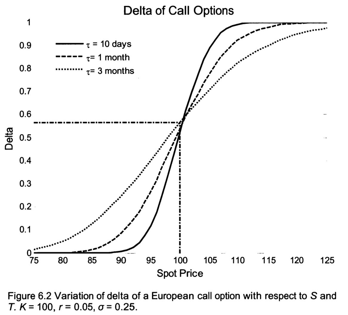
Delta: \(\Delta=\frac{\partial f}{\partial S}\)
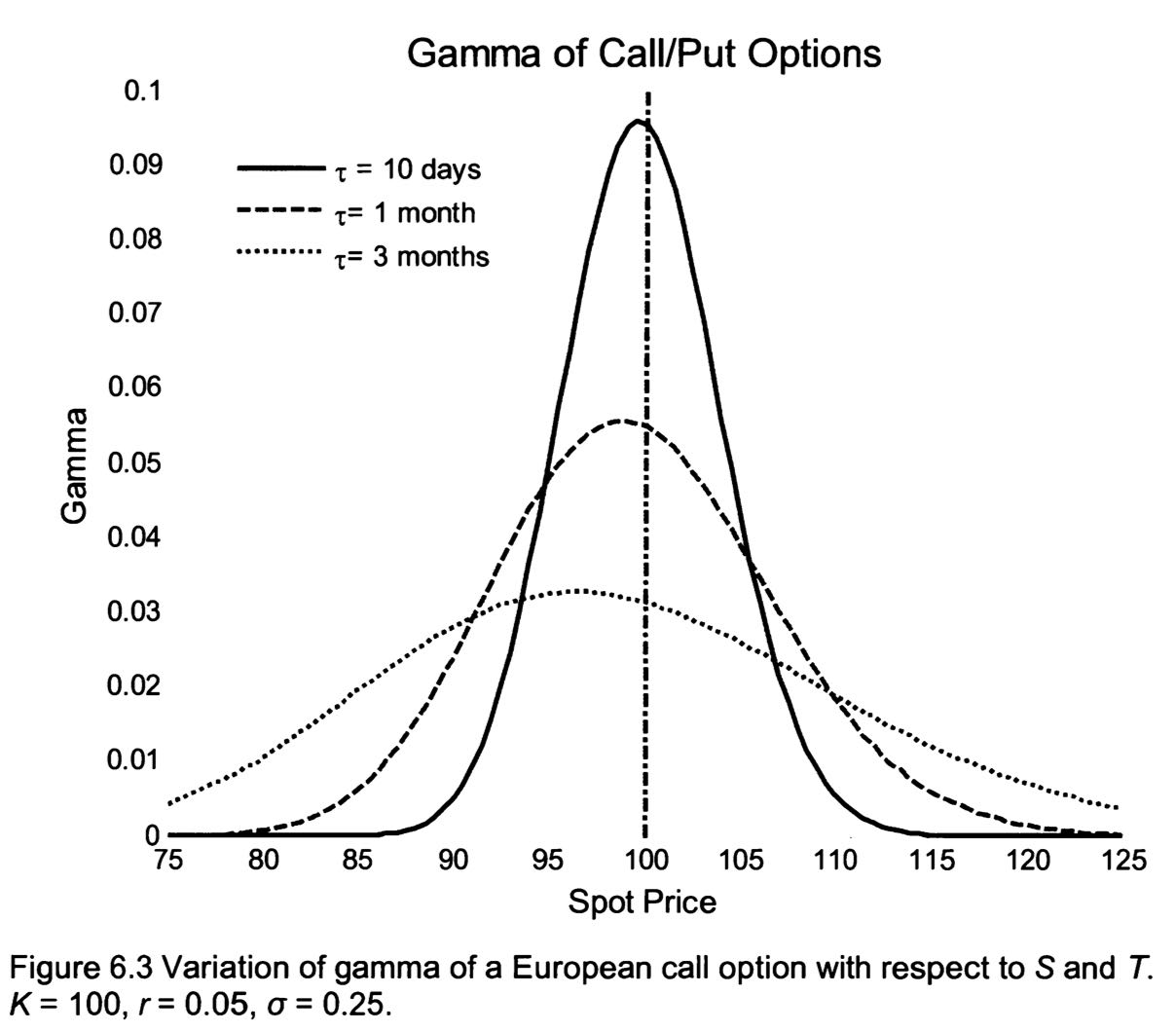
Gamma: \(\Gamma=\frac{\partial^{2} f}{\partial S^{2}}\)
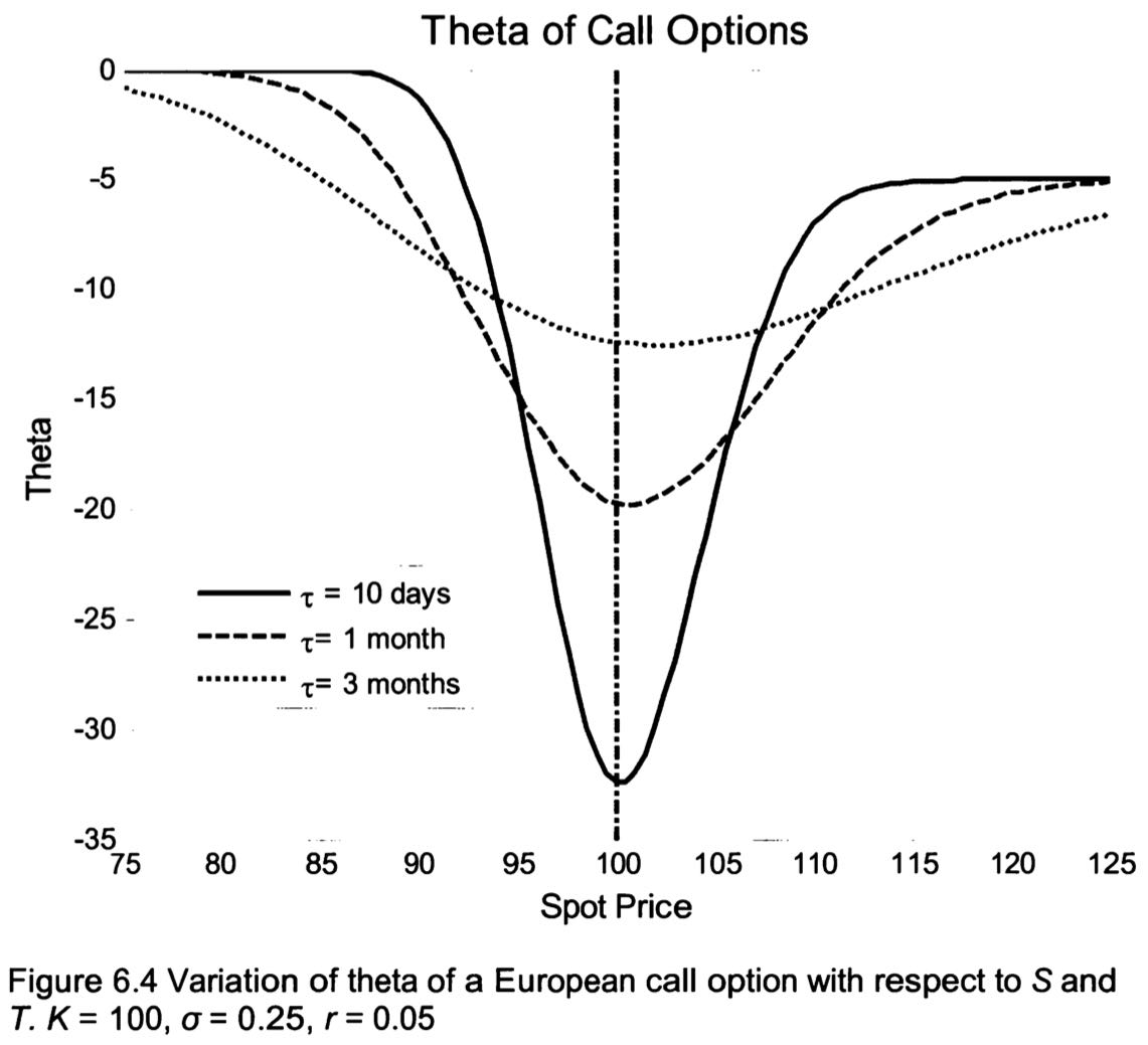
Theta: \(\Theta=\frac{\partial f}{\partial t}\)
Vega: \(\nu=\frac{\partial f}{\partial \sigma}\)
Rho: \(\rho=\frac{\partial f}{\partial r}\)
Delta
For a European call with dividend yield y: \[
\Delta=e^{-y \tau}N\left(d_{1}\right)
\] For a European put with dividend yield y: \[
\Delta=-e^{-y \tau}\left[1-N\left(d_{1}\right)\right]
\]
Delta Hedging
By BS PDE: \[ \theta^1 = \frac{\partial V}{\partial S} \]
- Delta Hedging only replicates the value and the slope of the option. To hedge the curvature of the option, need to hedge gamma as well.
Gamma
European call/put with dividend yield y: \[ \Gamma=\frac{N^{\prime}\left(d_{1}\right) e^{-y \tau}}{S_{0} \sigma \sqrt{\tau}} \]
- For plain vanilla call and put options, gamma is always positive
Gamma hedging
The delta hedge only replicates the value and the slope of the option. To hedge the curvature of the option, we will need to hedge gamma as well.
Theta
For a European call option: \[ \Theta=-\frac{S N^{\prime}\left(d_{1}\right) \sigma e^{-y \tau}}{2 \sqrt{\tau}}+y S e^{-y \tau} N\left(d_{1}\right)-r K e^{-r \tau} N\left(d_{2}\right) \]
For a European put option: \[ \Theta=-\frac{S N^{\prime}\left(d_{1}\right) \sigma e^{-y \tau}}{2 \sqrt{\tau}}-y S e^{-y \tau} N\left(-d_{1}\right)+r K e^{-r \tau} N\left(-d_{2}\right) \]
Vega
For European options: \[ v=\frac{\partial c}{\partial \sigma}=\frac{\partial p}{\partial \sigma}=S e^{-y \tau} \sqrt{\tau} N^{\prime}\left(d_{1}\right) \]
- Long-term option is more sensitive to change in volatility
Implied volatility:
- the volatility that makes the model option price equal to the market option price
Volatility smile:
- the relationship between the implied volatility of the options and the strike prices for a given asset.
Other options
- Bull spread:
- long 1 call/put with \(K_1\)
- short 1 call/put with \(K_2\)
- Straddle
- long 1 call option with K
- long 1 put option with K
Appendix
\[ \frac{\partial}{\partial z} \int_{a(z)}^{b(z)} f(x, z) d x=\int_{a(z)}^{b(z)} \frac{\partial f(x, z)}{\partial z} d x+f(b(z), z) \frac{\partial b}{\partial z}-f(a(z), z)\frac{\partial a}{\partial z} \]