Machine Learning Week09
Anomaly Detection 异常检测
Density Estimation
Problem Motivation
异常检测主要用于unsupervised learning
Model:\(P(x_{test}<\epsilon)\rightarrow anomaly\)
\(P(x_{test}\ge \epsilon)\rightarrow OK\)
也被用于检测账号被盗、生产、数据中心的电脑
Gaussian Distribution
=Normal distribution
X ~ N (0, 1),“distributed as”, 这里N的符号为"script N"
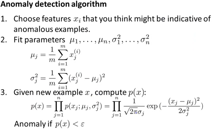
给定dataset,参数估计:via Maximum likelihood estimation 通常是m-1,对大数据集没影响 \[ \mu = \frac{1}{m}\sum_{i=1}^mx^{(i)}\\ \sigma^2=\frac{1}{m}\sum_{i=1}^m(x^{(i)}-\mu)^2 \]
Algorithm
基本假设,各特征间相互独立 \[
P(x)=\prod_{j=1}^np(x_j;\mu_j,\sigma_j^2)
\] 
Building an Anomaly Detection System
Developing and Evaluating an Anomaly Detection System
Training set: normal examples (可以有少量异常的混进来)
然后应用于cross calidation set 和 test set
10000正常,20异常:
训练集:6000正常
CV:2000正常,10异常
Test:2000正常,10异常
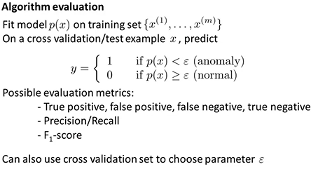
由于normal是0,所以预测0常常有更高的准确率,是skew的偏斜的。因此查准率accuracy不是很好的分析指标。
- 选择ε时,可以试几个不同的,然后选择使得Cross validation集中F1-score最大的,或者效果最好的。
- 有时还需要决定用什么特征
Anomaly detection vs. Supervised learning
Anomaly detection:
- y=1非常少(0-20常见), y=0占比更大
- 有大量不同的异常类型,其他算法难于分辨各种类型
- 有未知异常类型
supervised learning:
- 大量的positive 和negative examples
- 有足够positive examples,并且未来的positive example和训练集的相似
- Spam
Choosing what features to use
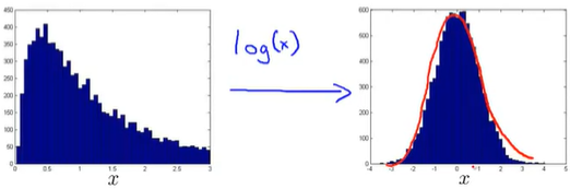
- Non-gaussian feature
绘制特征的直方图,看是否大致是个bell shaped curve,如果不是,运用一些变换使得其看起来更加gaussian
Error analysis for anomaly detection
甄别失败时,new feature 可能有帮助,例如组合现有的特征形成新特征
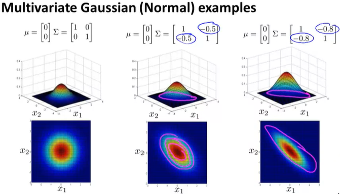
Multivariate Gaussian Distribution
Multivariate Gaussian Distribution
不同于之前的是,p(x)不再是各个特征概率的乘积。
Parameters: \(\mu \in \R^n\), \(\Sigma \in \R^{n\times n}\) \[ p(x;\mu,\Sigma)= \frac{1}{(2\pi)^{\frac{n}{2}}|\Sigma|^2}exp(-\frac{1}{2}(x-\mu)^T\Sigma^{-1}(x-\mu)) \] \(|\Sigma|\)=determinant of Σ
 \[
\mu = \frac{1}{m}\sum_{i=1}^mx^{(i)}\\
\Sigma = \frac{1}{m}\sum_{i=1}^m(x^{(i)}-\mu)(x^{(i)}-\mu)^T
\]
\[
\mu = \frac{1}{m}\sum_{i=1}^mx^{(i)}\\
\Sigma = \frac{1}{m}\sum_{i=1}^m(x^{(i)}-\mu)(x^{(i)}-\mu)^T
\]
Anomaly Detection using the multivariate Gaussian distribution
首先计算μ和Σ,然后计算p(x),最后根据ε判断是否异常
优点:自动捕捉特征间的相关性。m>10n用起来才比较好,必须要m>n,否则协方差矩阵不可逆。
缺点:计算量比较大。如果某个特征是其他的线性组合,那么协方差矩阵也不可逆,要注意避免。
前述的模型:优点在于计算量小,但是要人工创造一些新特征来更好地分辨。m<n的时候也能用。
若出现协方差矩阵不可逆:
- 首先检查m, n大小
- 检查是否有redundant features,就是特征间是否线性独立
Predicting Movie Ratings ——Recommendation System
Problem Formulation
r(i,j) 表示第i个电影,j用户是否打分;
y(i,j) 表示该用户对该电影的打分值 ;
Content Based Recommendations
设电影特征n个
For each user j, learn a parameter \(\theta^{(j)}\in\R^{n+1}\). Predict user j as rating movie i with \((\theta^{(j)})^Tx^{(i)}\) stars. (注意 \(x_0=1\))。用线性回归
To learn \(\theta^{(j)}\): \[ \min_{\Theta^{(j)}}\frac{1}{2m^{(j)}}\sum_{i:r(i,j)=1}((\theta^{(j)})^Tx^{(i)}-y^{(i,j)})^2+\frac{\lambda}{2m^{(j)}}\sum_{k=1}^{n}(\theta_k^{(j)})^2 \] Note: 这里 \(m^{(j)}\)可以去掉,对结果没有任何影响
优化目标也可以为: \[ J(\Theta^{(1)},...,\Theta^{(n_u)})=\min_{\Theta^{(1)},...,\Theta^{(n_u)}}\frac{1}{2}\sum_{j=1}^{n_u}\sum_{i:r(i,j)=1}((\theta^{(j)})^Tx^{(i)}-y^{(i,j)})^2+\frac{\lambda}{2}\sum_{j=1}^{n_u}\sum_{k=1}^{n}(\theta_k^{(j)})^2 \] Gradient descent update: \[ \theta_{k}^{(j)}:=\theta_{k}^{(j)}-\alpha \sum_{i: r(i, j)=1}\left(\left(\theta^{(j)}\right)^{T} x^{(i)}-y^{(i, j)}\right) x_{k}^{(i)}\ (\text { for } k=0) \]
\[ \theta_{k}^{(j)}:=\theta_{k}^{(j)}-\alpha\left(\sum_{i: r(i, j)=1}\left(\left(\theta^{(j)}\right)^{T} x^{(i)}-y^{(i, j)}\right) x_{k}^{(i)}+\lambda \theta_{k}^{(j)}\right)\ (\text { for } k \neq 0) \]
k=0的时候不加正则项
Collaborative Filtering
Collaborative Filtering
feature learning
Given \(\Theta^{(1)},...,\Theta^{(n_u)}\),to learn \(x^{(1)},...,x^{(n_m)}\);
算法类似7、8式
\(用户的\Theta\rightarrow 电影特征x\rightarrow \Theta\rightarrow x\rightarrow...\)
每个用户都在帮助这个推荐系统更好地分类电影,从而更好地预测评分
算法:同时实现:
Given \(x^{(1)},...,x^{(n_m)}\),estimate \(\theta^{(1)},...,\theta^{(n_u)}\): \[ \min_{\Theta^{(j)}}\frac{1}{2m^{(j)}}\sum_{i:r(i,j)=1}((\theta^{(j)})^Tx^{(i)}-y^{(i,j)})^2+\frac{\lambda}{2m^{(j)}}\sum_{k=1}^{n}(\theta_k^{(j)})^2 \]
Given \(\theta^{(1)},...,\theta^{(n_u)}\),estimate \(x^{(1)},...,x^{(n_m)}\): \[ \min _{x^{(1)}, \ldots, x^{\left(n_{m}\right)}} \frac{1}{2} \sum_{i=1}^{n_{m}} \sum_{j: r(i, j)=1}\left(\left(\theta^{(j)}\right)^{T} x^{(i)}-y^{(i, j)}\right)^{2}+\frac{\lambda}{2} \sum_{i=1}^{n_{m}} \sum_{k=1}^{n}\left(x_{k}^{(i)}\right)^{2} \]
即:
Minimizing \(x^{(1)},...,x^{(n_m)}\) and \(\theta^{(1)},...,\theta^{(n_u)}\) simultaneously: \[ \min_{x^{(1)},...,x^{(n_m)}\\\theta^{(1)},...,\theta^{(n_u)}}J\left(x^{(1)}, \ldots, x^{\left(n_{m}\right)}, \theta^{(1)}, \ldots, \theta^{\left(n_{u}\right)}\right) \]
\[ J\left(x^{(1)}, \ldots, x^{\left(n_{m}\right)}, \theta^{(1)}, \ldots, \theta^{\left(n_{u}\right)}\right)=\frac{1}{2} \sum_{(i, j): r(i, j)=1}\left(\left(\theta^{(j)}\right)^{T} x^{(i)}-y^{(i, j)}\right)^{2}+\frac{\lambda}{2} \sum_{i=1}^{n_{m}} \sum_{k=1}^{n}\left(x_{k}^{(i)}\right)^{2}+\frac{\lambda}{2} \sum_{j=1}^{n_{u}} \sum_{k=1}^{n}\left(\theta_{k}^{(j)}\right)^{2} \]
该算法下,无需设定 \(x_0=1\), 也没有\(\theta_0\),因为算法会自行选择参数。该算法下:\(\theta\in\R^n\),\(x\in\R^n\),n是特征数
算法实现:
- Initialize \(x^{(1)},...,x^{(n_m)}\), \(\theta^{(1)},...,\theta^{(n_u)}\) to small random values
- Minimize J using gradient descent (or an advanced optimization algorithm)
- For a user with parameters \(\theta\) and a movie with (learned) features x, predict a star rating of \(\theta^Tx\)
Low Rank Matrix Factorization
### Vectorization
Given matrices X (each row containing features of a particular movie) and Θ (each row containing the weights for those features for a given user), then the full matrix Y of all predicted ratings of all movies by all users is given simply by: \(Y = X\Theta^T\).
Predicting how similar two movies i and j are can be done using the distance between their respective feature vectors x. Specifically, we are looking for a small value of \(||x^{(i)} - x^{(j)}||\).
Mean Normalization
If the ranking system for movies is used from the previous lectures, then new users (who have watched no movies), will be assigned new movies incorrectly. Specifically, they will be assigned θ with all components equal to zero due to the minimization of the regularization term. That is, we assume that the new user will rank all movies 0, which does not seem intuitively correct. 新用户会被预测为0
We rectify this problem by normalizing the data relative to the mean. First, we use a matrix Y to store the data from previous ratings, where the ith row of Y is the ratings for the ith movie and the jth column corresponds to the ratings for the jth user.
We can now define a vector \[ \mu = [\mu_1, \mu_2, \dots , \mu_{n_m}] \] such that \[ \mu_i = \frac{\sum_{j:r(i,j)=1}{Y_{i,j}}}{\sum_{j}{r(i,j)}} \] Which is effectively the mean of the previous ratings for the ith movie (where only movies that have been watched by users are counted). We now can normalize the data by subtracting u, the mean rating, from the actual ratings for each user (column in matrix Y):
As an example, consider the following matrix Y and mean ratings μ: \[ Y=\left[\begin{array}{cccc} 5 & 5 & 0 & 0 \\ 4 & ? & ? & 0 \\ 0 & 0 & 5 & 4 \\ 0 & 0 & 5 & 0 \end{array}\right], \quad \mu=\left[\begin{array}{c} 2.5 \\ 2 \\ 2.25 \\ 1.25 \end{array}\right] \] The resulting Y′ vector is: \[ Y^{\prime}=\left[\begin{array}{cccc} 2.5 & 2.5 & -2.5 & -2.5 \\ 2 & ? & ? & -2 \\ -2 .25 & -2.25 & 3.75 & 1.25 \\ -1.25 & -1.25 & 3.75 & -1.25 \end{array}\right] \] Now we must slightly modify the linear regression prediction to include the mean normalization term: \[ (\theta^{(j)})^T x^{(i)} + \mu_i \] Now, for a new user, the initial predicted values will be equal to the μ term instead of simply being initialized to zero, which is more accurate.
Note: 一般的均值归一化要除以range,即max-min,但是这里不需要,因为都有统一的scale