Machine Learning Week08
Unsupervised learning 无监督学习
Clustering 聚类
无监督学习是不给分类标签y
1. 应用:
- 对消费者市场划分
- 社交网络分析
- 管理计算机
- 获取星系信息
2. K-means algorithm K均值算法
随机选择两个点作为聚类中心(分两类),然后进行下面两步
- 簇分配,遍历每个点,和哪个cluster centroid更近
- 移动聚类中心到上面分配的簇的均值
Input:
- K - number of clusters
- training set
algorithm
1
2
3
4
5
6
repeat{
for i=1 to m
c_i := index (from 1 to K) of cluster centroid closest to x_i
for k=1 to K
u_k := average (mean) of points assigned to cluster k
}如果有中心没有被分配到任何点,可以删去这个分类,也可以reinitialize the cluster centroid
3. K-means for non-sperated clusters
- 根据身高体重分类T恤大小
4. Optimization Objective
\[ \begin{array}{l} J\left(c^{(1)}, \ldots, c^{(m)}, \mu_{1}, \ldots, \mu_{K}\right)=\frac{1}{m} \sum_{i=1}\left\|x^{(i)}-\mu_{c^{(i)}}\right\|^{2} \\ \min _{c^{(1)}, \ldots, c^{(m)},\mu_{1}, \ldots, \mu_{K}} J\left(c^{(1)}, \ldots, c^{(m)}, \mu_{1}, \ldots, \mu_{K}\right) \end{array} \]
also called distortion of K-means algorithm
cost function 关于iteration的曲线
5. Random Initialization
随机初始化聚类中心
随机选k个个例本身,作为中心,但是容易陷入Local optima。解决方案:多次随机,选择cost function最小的
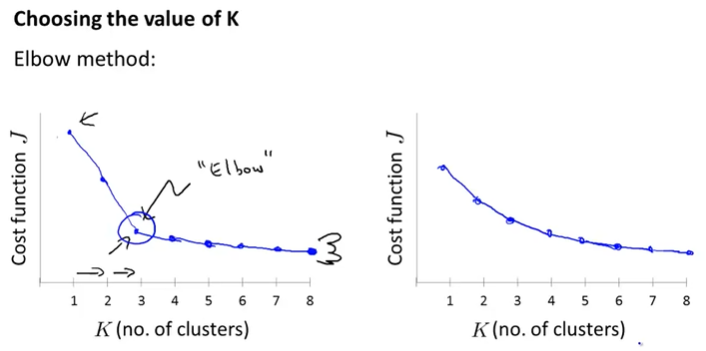
6. Choosing the Number of Clusters
Elbow Method:
绘制J关于K的曲线,找到“Elbow”的节点,作为分类个数
用途之一:later/downstream purpose
Motivation
1. Data Compression ---- Dimensionality Reduction降维
压缩数据,减少内存占用加快运算
2. Data Visualization
降维可以便于数据可视化
Principal Component Analysis主成分分析
1. Problem formulation
PCA:To find a surface onto which to project the data so as to minimize the the projection error (线性拟合中就是使得离某条直线的距离最小).
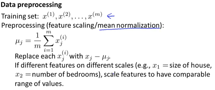
- 先mean normalization(feature scaling)
- Reduce from 2-dimension to 1-dimension: Find a direction (a vector \(u_i\in \R^n\)) onto which to project the data so as to minimize the projection error. 该向量的正负没有关系。
- Reduce from n-dimension to k-dimension: Find k vectors \(u^{(1)}\),\(u^{(2)}\), ... , \(u^{(k)}\) onto which to project the data so as to minimize the projection error.
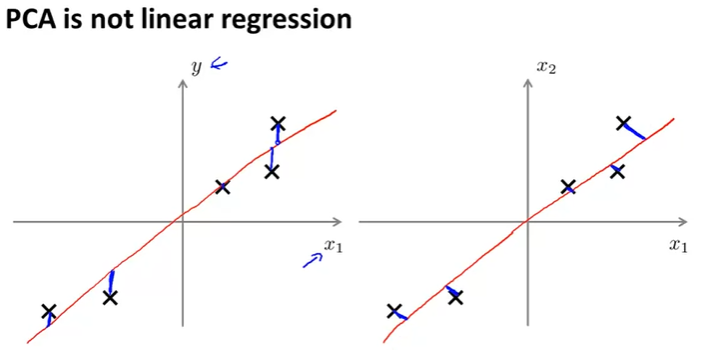
- 注:PCA is not linear regression。注意看下图区别,线性回归是和预期值的差最小,PCA是到直线距离最小
2. PCA Algorithm
PCA的目标:
- maximize variance perspective 最大投影方差
- minimize error perspective 最小重构代价
Step1: mean normalization. 根据数据(有不同的scales),可能还需要feature scaling。均值归一化是特征缩放的一种方法。(除以标准差)
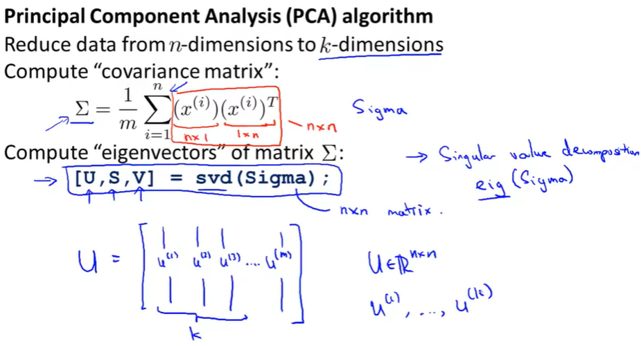
Step2: Reduce data from n-dimensions to k-dimensions:
Compute "covariance matrix": \(\Sigma = \frac{1}{m}\sum_{i=1}^{n}{(x^{(i)})(x^{(i)})^T}\),xi是n*1的列向量,symmetric positive definite
Compute "eigenvectors" of matrix \(\Sigma\): [U, S, V] = svd(Sigma) ;或者 eig(Sigma)
svd: Singular value decomposition 奇异值分解
其中U是我们需要的, 列向量为各个特征向量,压缩到k个向量只需要取前k个列向量(对称矩阵的特征向量是正交的)
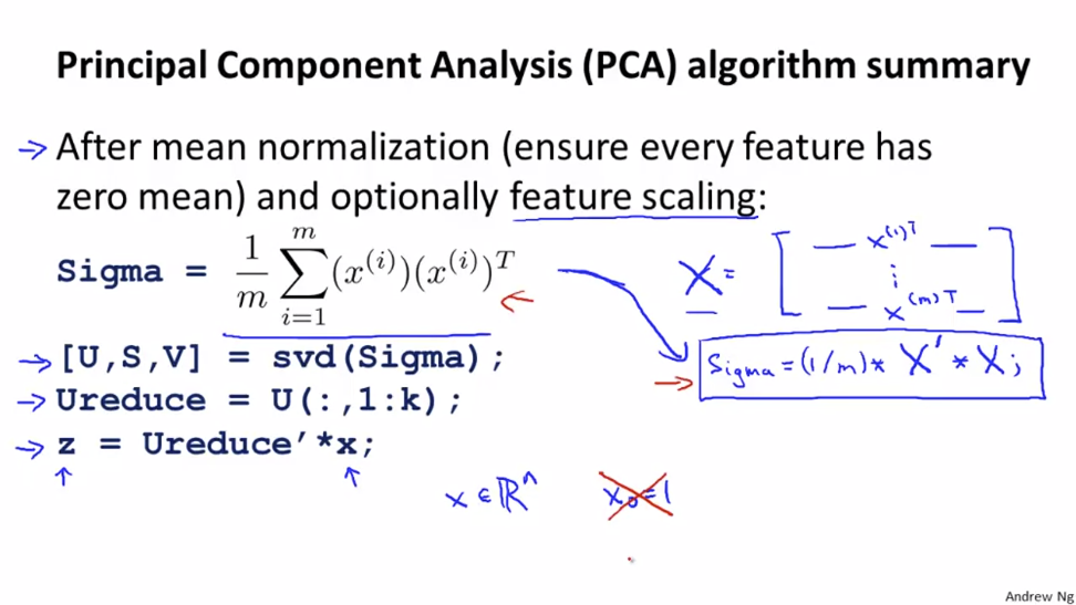
注:PCA算法中,没有x0=1这一项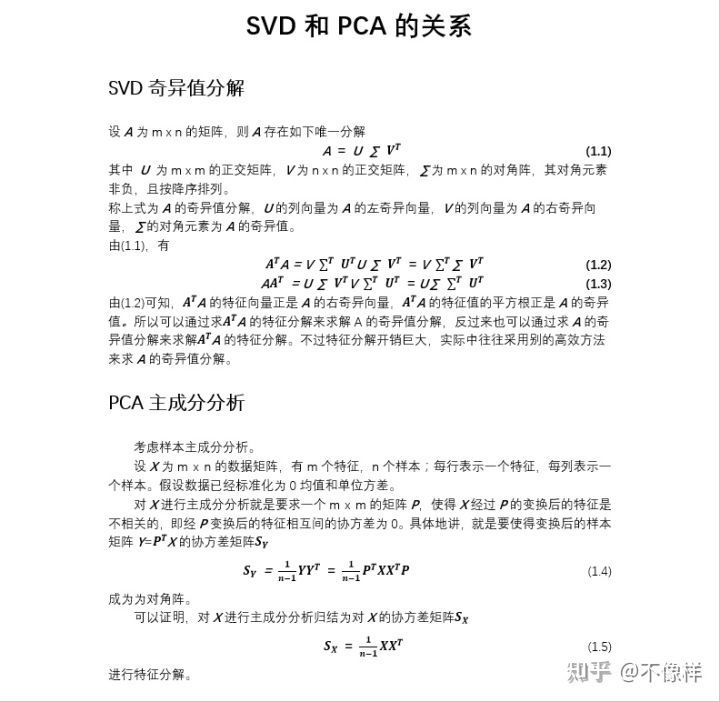
疑问:
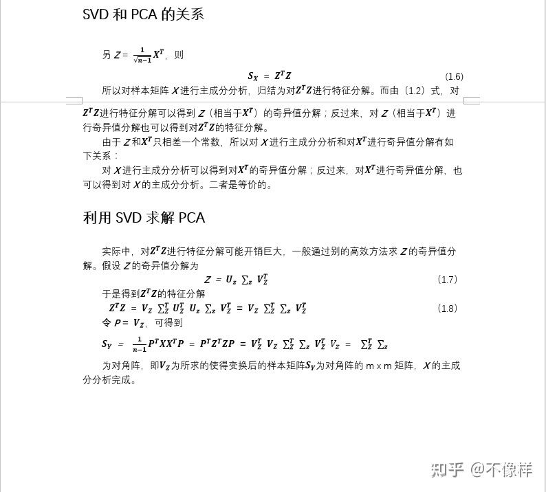
为什么不直接用X进行SVD,而要算协方差的SVD?
Answer:协方差的U和X的V是相等的,其实都可以
理解:\(X=U'S'V'^T\), \(X^TX=USV^T\),现要说明 \(V'=U\), 只需要 \(X^TX=V'S'^2V'^T=USV^T\),所以 \(V'=U\)。
为什么要取协方差矩阵SVD后的左奇异矩阵来压缩特征维度?
首先易证一个SPD矩阵通过SVD得到的U和V是相等的。
其次,通常我们用XV=YU来表示坐标变换。
\(\Sigma = X^TX\),又有 \(\Sigma = USV^T\),可以得到 \(\Sigma V = US\),这里实际上是将covariance矩阵变化为对角线矩阵,即互不相关(其中U=V,即U为协方差矩阵的特征向量,S为其特征值)。那么这时,我们令XI=UZ,I是X坐标系下的正交基,即 \(Z=U^TX\)。此时Z的协方差 \(Z^TZ=\Sigma\)。
Applying PCA
Reconstruction from compressed representation
\[ z=U_{reduce}^Tx \]
可以得到: \[ x_{approx}=U_{reduce}z \]
Choosing the number k of principal component
- Average squared projection error:
\[ \frac{1}{m}\Sigma_{i=1}^m\parallel x^{(i)}-x_{approx}^{(i)}\parallel ^2 \]
Tptal variation in the data: \[ \frac{1}{m}\Sigma_{i=1}^m\parallel x^{(i)}\parallel ^2 \]
Choose k to be smallest value so that \[ \frac{\frac{1}{m}\Sigma_{i=1}^m\parallel x^{(i)}-x_{approx}^{(i)}\parallel ^2}{\frac{1}{m}\Sigma_{i=1}^m\parallel x^{(i)}\parallel ^2}\le0.01 \] "99% of variance is retained"。这个数值可以根据需求不同更换。
算法:
SVD函数返回的S矩阵为diagonal matrix。
For given k: k 递增,使得 \[ 1-\frac{\Sigma_{i=1}^{k}S_{ii}}{\Sigma_{i=1}^{n}S_{ii}}\le0.01 \]
选择最小的K满足上式。
根据性质:矩阵特征值之和等于主对角线元素之和,易证(6)式等价于(7)式。
Advice for applying PCA
Supervised learning speedup
压缩原始训练集数据的维度
Mapping \(x^{(i)}\rightarrow z^{(i)}\)should be defined by running PCA only on the trainning set. This mapping can be applied as well to the examples \(x_{CV}^{(i)}\) and \(x_{test}^{(i)}\) in the cross validation and test sets.
Compression
- Reduce memory/disk needed to store data
- speed up learning algorithm
Visualization
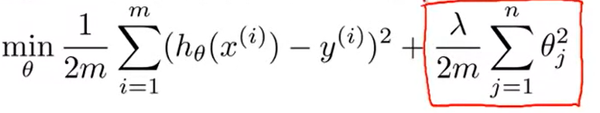
Bad use of PCA: To prevent overfitting
可能确实可以避免过拟合,但是不是解决过拟合的好方法。正确方法式加正则项(Use regularization instead!)
For example:
正确做法是先不用PCA,在原始数据跑一遍,如果不符合期望,再用PCA